Faster R-CNN step by step, Part I
Faster R-CNN is a good point to learn R-CNN family, before it there have R-CNN and Fast R-CNN, after it there have Mask R-CNN.
In this post, I will implement Faster R-CNN step by step in keras, build a trainable model, and dive into the details of all tricky part.
Before start, I suppose you already known some convolutional neural network, objection detection and keras basics.
Overview
Faster R-CNN can be generally divided into two parts, RPN part and R-CNN part, each part is an independent neural network and can be trained jointly or separately. To better explanation, I will implement and train those two part separately, for this first article, let’s focus on RPN part. I will break down this post to several sections.
- RPN model architecture.
- How to prepare data to train RPN.
- Loss function.
- Use trained RPN to predict proposals.
the code in this post can be found in this link, some code are copied form rbg’s implementation and broadinstitute/keras-rcnn.
RPN model
RPN is stand for Region Proposal Network. When I first learn Faster R-CNN, this RPN conception sounds very difficult to me, there have a lot of trick things like feature map, anchors, etc, but actually RPN is just another simple neural network, we can see how simple this network is, the implementation look like below.
feature_map_tile = Input(shape=(None,None,1536))
convolution_3x3 = Conv2D(
    filters=512,
    kernel_size=(3, 3),
    name="3x3"
)(feature_map_tile)

output_deltas = Conv2D(
    filters= 4 * k,
    kernel_size=(1, 1),
    activation="linear",
    kernel_initializer="uniform",
    name="deltas1"
)(convolution_3x3)

output_scores = Conv2D(
    filters=1 * k,
    kernel_size=(1, 1),
    activation="sigmoid",
    kernel_initializer="uniform",
    name="scores1"
)(convolution_3x3)

model = Model(inputs=[feature_map_tile], outputs=[output_scores, output_deltas])
Like the code shown, RPN is a simple 3 layer neural network, let’s take a close look at the layers.
input layer
Input part is a shape of feature map, too make a clear explain, let’s call the input 1st layer feature map, the details of feature map will describe later.
3x3 conv layer
The second layer is a 3x3 convolutional layer, this layer is controlling receptive field, each 3x3 tile in 1st layer feature map will map to one point in output feature map, in another word, each point of output is representing (3, 3) block of 1st layer feature map and eventually to a big tile of original image. to distinguish with 1st layer feature map, let’s call the output 2nd layer feature map, point in the feature map is called feature map point, each point have shape (1,1,1532).
two head output
Following the second layer, there have two sibling output layers, first one have 1*9 unit output, here 9 is the anchor number, we will come to anchors later, now just consider 9 as a constant, 1*9 represent the label of of each anchor, 1 mean the anchors proposal region is foreground, 0 is background, -1 means ignore this anchor. The second output have 4*9 units, which represent the bounding boxes of anchors, 4 values are NOT $x_{min},y_{min},x_{max},y_{max}$, it is transformed to calculate loss function.
Faster R-CNN Paper described this architecture, very neat.
the fully-connected layers are shared across all spatial locations. This architecture is naturally implemented with an n×n convolutional layer followed by two sibling 1 × 1 convolutional layers (for reg and cls, respectively).
Training data produce
Now we have an intuition about RPN model and it’s input and output, but how to prepare training data? This is probably the most tricky part of RPN.
Let us recall classical image classification model, we usually scale several images to same size and feed them as a mini-batch to model, and expect a category output. In RPN it is different, no need scale image, and no multi image one batch, it will produce a batch of training data base on a single image, this is called “image-centric” sampling strategy.
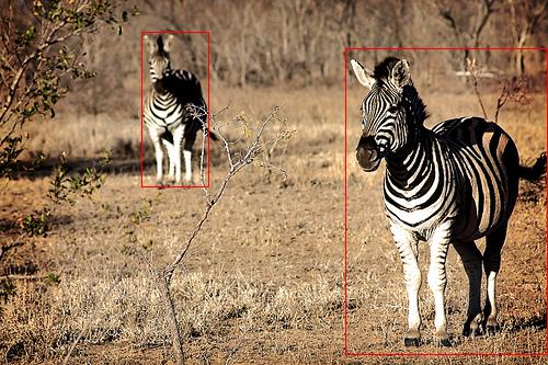
In rbg’s implementation, he feed an image feature map to model and there have a anchor_target_layer to break that image down to many data, and then randomly choose 256 data to form a mini-batch. In this article, I will split image feature map and form mini-batch firstly and feed to model, the trick part is then move from model training phase to data preprocessing phase. I will use one image from ILSVRC2014 to show how to break down image into a mini batch of data, and train RPN model.
the image have shape (333, 500, 3) and two ground truth boxes.
pretrained model and feature map
RPN use pre-trained CNN models to extract image features, the 1st layer feature map, here I use InceptionResNetv2 as pre-trained model, the shape of the feature map is (height, width, 1532), feature map height and width is not fixed because image height and width is fixed.
pretrained_model = InceptionResNetV2(include_top=False)
feature_map=pretrained_model.predict(x)
by feeding the 333x500 image, we have a 1st layer feature map with shape (9, 14, 1532). the 2nd layer feature map have same shape.
calculate stride
With the feature map, we can calculate the overall stride between feature map with shape (9, 14, 1532) and original image with shape (333, 500, 3)
w_stride = img_width / width
h_stride = img_height / height
In Faster R-CNN paper, the pre-trained model is VGG16 and the stride is (16, 16), here because we are using InceptionResNetV2, the stride for height and width is not fixed and will change from image to image, for this 333x500 image, we have stride (37, 35.7).
With the stride, we can split original image into many tiles.
shift_x = np.arange(0, width) * w_stride
shift_y = np.arange(0, height) * h_stride
shift_x, shift_y = np.meshgrid(shift_x, shift_y)
shifts = np.vstack((shift_x.ravel(), shift_y.ravel(), shift_x.ravel(),
                        shift_y.ravel())).transpose()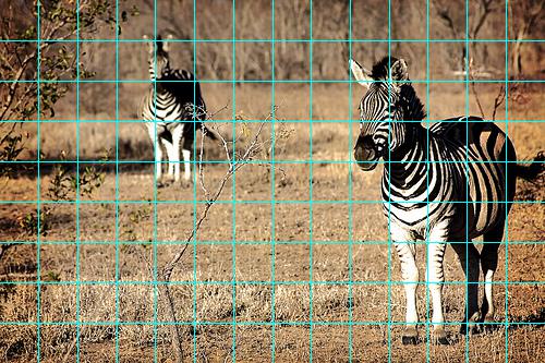
NOTE: Those tiles are just utilized to create anchors, not means a feature map point receptive field is same as a tile, actually 1st layer feature map point have much bigger receptive field than the tile, in VGG16, each 1st layer feature map point have a (192,192) size image tile mapped as a receptive field, the 2nd layer feature map point have even bigger receptive field.
generate anchors for one point
After we have the tiles, we can now introduce anchors. For each tile, there have several fixed size and shape box draw on it, like below.
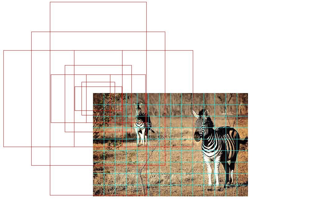
those boxes are called “anchors”, anchors are pre-defined and not trainable.
the number, shape and size of anchors can tune manually, in this example, I use scale (3,6,12) instead of (8,16,32) in Paper, because the stride and receptive field is bigger than VGG16 in Paper, so need smaller scale to get finer anchor boxes, I use 9 anchors for each tile.
generate anchors for all point
when apply anchors to all tile
base_anchors=generate_anchors(w_stride,h_stride)
all_anchors = (base_anchors.reshape((1, 9, 4)) +
                shifts.reshape((1, num_feature_map, 4)).transpose((1, 0, 2)))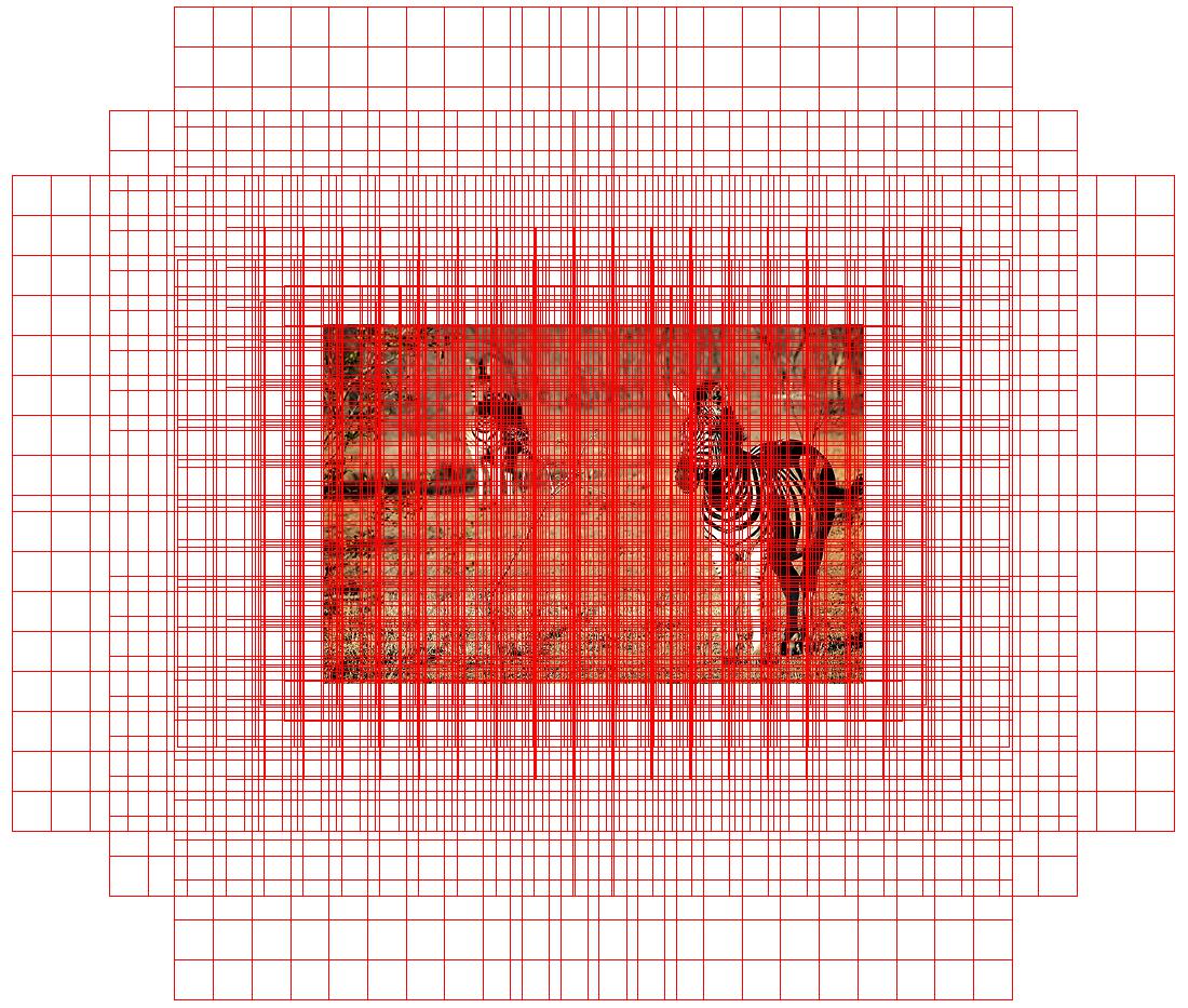
there are huge number of anchors.
remove anchors not inside image.
border=0
inds_inside = np.where(
        (all_anchors[:, 0] >= -border) &
        (all_anchors[:, 1] >= -border) &
        (all_anchors[:, 2] < img_width+border ) &  # width
        (all_anchors[:, 3] < img_height+border)    # height
)[0]
anchors=all_anchors[inds_inside]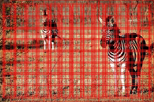
get overlaps and set label.
Use IoU to calculate overlaps between anchors and ground true boxes(gt boxes). in Paper, the rule to set positive are defined:
We assign a positive label to two kinds of anchors: (i) the anchor/anchors with the highest Intersection-overUnion (IoU) overlap with a ground-truth box, or (ii) an anchor that has an IoU overlap higher than 0.7 with any gt boxes
#labels, 1=fg/0=bg/-1=ignore
labels = np.empty((len(inds_inside), ), dtype=np.float32)
labels.fill(-1)
labels[gt_argmax_overlaps] = 1
labels[max_overlaps >= .7] = 1
labels[max_overlaps <= .3] = 0
subsample labels
the fg/bg numbers could be much bigger than a batch size(e.g. 256), so need randomly down sample, also bg samples number is much bigger than fg samples, that will make bias towards bg samples, so need keep fg/bg ratio. below is fg sample example code, bg sample is similiar.
# subsample positive labels if we have too many
num_fg = int(RPN_FG_FRACTION * RPN_BATCHSIZE)
fg_inds = np.where(labels == 1)[0]
if len(fg_inds) > num_fg:
    disable_inds = npr.choice(
        fg_inds, size=(len(fg_inds) - num_fg), replace=False)
    labels[disable_inds] = -1
after this step, we have fix size anchors batch, with 1:3 fg/bg ratio.
prepare mini batch data
with the down sampled anchors, we now need calculate feature map point position for each anchor sample, and use that position to form our mini-batch. for example, an anchor sample have index 150, divided by 9, get integer 16, this 16 represented a point (1,2), the second row, third column point in feature map.
batch_inds=inds_inside[labels!=-1]
batch_inds=(batch_inds / k).astype(np.int)
when we got all mini batch related feature map point locations, it’s easy to prepare label and bounding box batch, each point correlated to 9 base anchors. target label batch have shape (batch_size, 1, 1, 9), target bounding box batch have shape (batch_size, 1, 1, 4*9), those targets will be used in two sibling outputs.
To prepare the inputs, let’s recall the second layer in mode, it is a 3x3 convolutional layer, when feature map point location “back propagate” to this layer, a point become to a 3x3 tile, so we need prepare a 3x3 tile batch as our input data, each tile is partial of 1st layer feature map.
# generate batch feature map 3x3 tile from batch_inds
padded_fcmap=np.pad(feature_map,((0,0),(1,1),(1,1),(0,0)),mode='constant')
padded_fcmap=np.squeeze(padded_fcmap)
batch_tiles=[]
for ind in batch_inds:
    x = ind % width
    y = int(ind/width)
    fc_3x3=padded_fcmap[y:y+3,x:x+3,:]
    batch_tiles.append(fc_3x3)
NOTE, in this implementation I did not sort the batch indexes, so different samples may correlated to a same location, cause some duplicate training data in mini batch.
Now we have input and targets. we need one more thing to do, define the loss function.
Loss function
In Paper, loss function is defined like below
\[L(p_i,t_i)=\frac{1}{N_{cls}}\sum{L_{cls}(p_i,p_i^*)}+\lambda\frac{1}{N_{reg}}p_i\sum{L_{reg}(t_i,t_i^*)}\]it combines loss function of label part and bounding box part, in the code, to make it easy, I removed some part like $\lambda$ and normalization.
model.compile(optimizer='adam', loss={'scores1':'binary_crossentropy', 'deltas1':'mse'})start train
now we can train the model with batch data.
model.fit(np.asarray(batch_tiles), [batch_label_targets,batch_bbox_targets], epochs=100)Predict proposal region
RPN is used separately to propose regions, feed an any size image to RPN, it will generate height*width*9 outputs, each output have two siblings, one is score between [0,1] represent probability of fg/bg, and another is 4 transformed values, we need do some work to process this output to bounding box proposals.
In the next part, let’s see how the use RPN predict result to do the real object detection task.