Faster R-CNN step by step, Part II
In last post, we saw how to implement RPN, the first part of Faster R-CNN, in this post, let’s continue to implement the left part, Region-based Convolutional Neural Network(R-CNN).
Overview
R-CNN is a first introduced by Girshick et al., 2014, it use selective search to propose 2000 region of interests(RoIs), and feed each 2000 RoIs to pre-trained CNN(e.g. VGG16) to get feature map, and predict the category and bouding box. Fast R-CNN then improve this procedure, instead of feed pre-trained CNN 2000 times, Fast R-CNN put them all together, and go though pre-trained CNN once. Faster R-CNN improve the selective search part by using RPN, dramatically improved the region proposal performance, which we’ve seen in last post.
This time we will take a look at Fast R-CNN, because Faster R-CNN is using same architecture in the R-CNN part.
I will break down this post to several sections.
- R-CNN model architecture.
- How use RPN generated RoIs to train R-CNN.
- Loss function and train
- Predict category and bounding box.
the code in this post can be found in this link, some code are copied form rbg’s implementation and broadinstitute/keras-rcnn.
R-CNN model
R-CNN model is another neural networks, like RPN, it has two heads,
feature_map=Input(batch_shape=(None,None,None,1536))
rois=Input(batch_shape=(None, 4))
ind=Input(batch_shape=(None, 1),dtype='int32')

p1=RoIPooling()([feature_map, rois, ind])

flat1 = Flatten()(p1)

fc1 = Dense(
        units=1024,
        activation="relu",
        name="fc2"
    )(flat1)

output_deltas = Dense(
        units=4 * 200,
        activation="linear",
        kernel_initializer="uniform",
        name="deltas2"
    )(fc1)

output_scores = Dense(
        units=1 * 200,
        activation="softmax",
        kernel_initializer="uniform",
        name="scores2"
    )(fc1)

model=Model(inputs=[feature_map, rois, ind],outputs=[output_scores,output_deltas])
The architecture is a little bit more complex than RPN, the tricky part is first layer RoI pooling layer.
input layer and RoI pooling layer
RoI pooling is a concept introduced by Fast R-CNN, basically it like max pooling but is pool non-fixed size boxes to a fixed size, so that next fully connected layer can use the output. this article have good animation for RoI pooling, RoI pooling layer is like a data shape normalizer, before it, the input is non-fixed size, after it, it have fixed size, let’s take a close look at the shape from beginning to end.
RoI pooling inputs
- feature map, this input have shape (feature map number, height, width, channels), as we see the first 3 shapes are not fixed, to make implementation easy, we use one feature map for each batch, in paper and rbg’s implementation also use one feature map each batch, reason is if use multiple feature map, the height and width of each feature map are not same, so need padding the feature map to same size, this may not easy.
- rois, have shape(None, 4), this part comes from RPN, with some processing to reduce the roi box number, usually this part have fixed size rois number, but for some reason the RPN will not produce enough rois to feed, so here the first dim is
None. - index, have shape(None, 1), this input indicate which feature map those rois are belong to, as we only have one feature map each batch, the index are always 0. the number is same as rois number.
RoI pooling output
The output shape is fixed, (None, 7, 7, 1536), the first dim have same number of rois, means each rois will produce a (1, 7, 7, 1536) tensor, and double 7 is defined by RoI pooling, 1536 is feature map channel size.
we can see in the output, batch size become fixed which is the equal to the number of rois, in this point our neural network can do what we want to do.
flatten layer
flatten data from convolutional style to dense style
dense layer
just dense
two heads
two sibling heads, one is one hot category, and another one is “one hot” bounding box.
Prepare traning data.
Now we have RCNN model, we can see the most important input is region of proposals(rois), other two inputs are feature map and its index which only have one value each batch, we will not explain too much on them.
To start, let’s first think some questions about rois:
- Where are rois come from? In Fast RCNN, it comes from a method called selective search, in Faster RCNN it comes from RPN layer.
- What is the number of rois? Faster R-CNN Paper describe this, in training phase, the number is 2000, in predict phase, it have several variants from 100-6000
- What is the format of rois? Simple $x_{min},y_{min},x_{max},y_{max}$ format.
Those Q/A explained some basics of rois, and to make the section clear, we split the data preprocessing into two parts, post RPN part and preprocessing of RCNN part
post RPN
From last post, the output of RPN have two heads, one is shape=(height, width, anchor_num * 4) bounding box, and one is shape=(height, width, anchor_num), those two outputs will be used to generate rois.
# feed feature map to pre-trained RPN model, get proposal labels and bboxes.
res=rpn_model.predict(feature_map)
scores=res[0]
scores=scores.reshape(-1,1)
deltas=res[1]
deltas=np.reshape(deltas,(-1,4))
transform format
For easy to regression, the bounding box output use transformed format, here we need transform them back to ‘box’ format: $x_{min},y_{min},x_{max},y_{max}$.
proposals =bbox_transform_inv(all_anchors, deltas)let’s take a look at the “raw” rois.
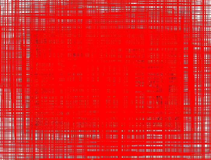
Looks crazy, need some steps to reduce the numbers.
clip box to image and remove small size box
proposals = clip_boxes(proposals, (h_w[0],h_w[1]))
keep = filter_boxes(proposals, 40)
proposals = proposals[keep, :]
scores = scores[keep]
keep to 6000 before non-maximum suppression
In this step, the rois size is not fixed, it depends on image height and width and upper two steps, this steps and following step are used to make its size fixed.
Remember in RPN output we have two heads? here the scores are used, scores are representing the confidence of rois to be a foreground or background object, in this step sort the scores and keep top 6000.
# sort scores and only keep top 6000.
pre_nms_topN=6000
order = scores.ravel().argsort()[::-1]
if pre_nms_topN > 0:
order = order[:pre_nms_topN]
proposals = proposals[order, :]
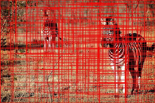
scores = scores[order]non-maximum suppression, and keep top 300.
Non-maximum suppression(nms) is an algorithm to reduce overlap rois,
In this step the post RPN processing is finished, usually this is a part of RPN, but too keep RPN clear I move it in this post and right before RCNN pre-processing.
If we draw those rois, it still mess, so I choose some of them which performs good proposal.
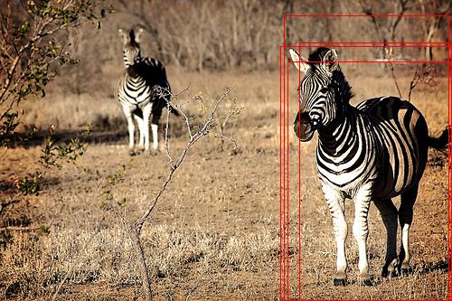
# apply NMS to to 6000, and then keep top 300
post_nms_topN=300
keep = py_cpu_nms(np.hstack((proposals, scores)), 0.7)
if post_nms_topN > 0:
    keep = keep[:post_nms_topN]
proposals = proposals[keep, :]
scores = scores[keep]
The final rois, look much clearer.
RCNN preprocessing
With last step output, we can think like this way: RPN and it’s post process give a fixed size usable rois, now let’s see how to process them to training data.
calculate overlap
This part is almost the same action we did in RPN, the purpose of this part is also same with RPN: given a set of boxes(for RPN the boxes are anchors, for RCNN the boxes are rois), calculate overlap of those boxes to ground truth boxes, and select qualified boxes base on the overlap value.
# add gt_boxes to proposals.
proposals=np.vstack( (proposals, gt_boxes) )
# calculate overlaps of proposal and gt_boxes
overlaps = bbox_overlaps(proposals, gt_boxes)
select rois with fg/bg ratio
if fg_inds.size > 0:
    fg_inds = npr.choice(fg_inds, size=fg_rois_per_this_image, replace=False)
if bg_inds.size > 0:
    bg_inds = npr.choice(bg_inds, size=bg_rois_per_this_image, replace=False)
keep_inds = np.append(fg_inds, bg_inds)
rois = proposals[keep_inds]
produce targets (bounding box and categories)
assign gt box to each rois, calculate the regression format, and put into right shape.
Loss function
RCNN combine two losses: classification loss which represent category loss, and regression loss which represent bounding boxes location loss.
classification loss is a cross entropy of 200 categories.
regression loss is similar to RPN, using smooth l1 loss. there have 800 values but only 4 values are participant the gradient calculation.
Summary
In this two posts, we have learnt how to implement Faster R-CNN step by step, how to prepare training data.
In order to make implementation easy to explain, In my implementation I assume the pre-trained CNN model(here is InceptionResNetV2) is fixed and not trainable, but in Paper those two networks will keep pre-trained CNN model updated, and the training process is alternating, which means RPN updated pre-trained model will be used in RCNN, and RCNN updated pre-trained model will be used in RPN, repeat this process to make model imporve.
Beside train separately, the Paper also describe a joint way to RPN and RCNN together, rbg’s implementation is using this method, it only have approximate result but more faster than separate training.
Consider those training methods, Faster RCNN is actually a complex algorithm to implement, in this two posts, I make some assumption to make implementation easier to understand, the overall algorithm is same as it’s in Paper.
Both RPN and RCNN have a simple network architecture but the data have non-fixed size and some tricks are used to processing data, those parts are the complex parts of Faster RCNN.
If you have any questions or comments, you can create an issue in code base.